EEG and Epilepsy: Binary Classification
Table of Contents
Introduction #
Overview #
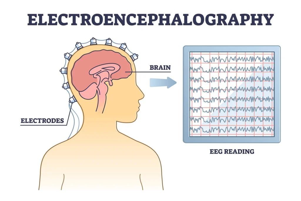
Epilepsy, also known as seizure disorder, is a medical condition characterized by recurring seizures due to abnormal electrical activity in the brain. In the United States, epilepsy affects almost 3 million adults. There are many ways to detect epileptic behavior in the brain, including electroencephalogram (EEG), magnetic resonance imaging (MRI), and computed tomography (CT) scans.
However, what makes EEG such a popular method to measure brain activity is its excellent temporal resolution, relatively low cost, and noninvasive nature. It is able to measure brain activity by recording electrical activity through a patient’s skull and scalp. Despite this, symptoms of epilepsy are not guaranteed to be present at all times of data collection. Thus, this process can take long periods of monitoring, generating large amounts of data.
Motivation #
Our motivation for this project is to be able to automate the process of identifying abnormality within brain activity patterns of EEG data, making the process to diagnosis of epilepsy faster for patients.
Automation with identification of EEG is especially important because of some difficulties when dealing with EEG, burdening experts and reducing efficiency:
- There are small amounts of epilepsy data available simply due to the infrequency of seizure occurences.
- Presence of noise and artifacts in the data disturbs learning brain patterns during ictal cases.
- Inconsistency in seizure activitation among different patients also hinders pattern learning.
Following a structured data science pipeline, our objective is to build a binary classification model to determine whether or not a patient is epileptic given EEG data.
Data #
Our data is sourced from hospital EEG recordings of healthy and epileptic patients, recorded across five electrode channels. The exact electrode channels are as follows:
- A1: Placed on the left ear to measure the average of all electrodes
- C3: Placed on the left primary motor cortex, measures motor movement of the right hand
- C4: Placed on the right primary motor cortex, measures motor movement of the left hand
- CZ: Placed on the center top of the head, measures possible temporal lobe epilepsy
- F3: Placed on the left frontal lobe, measures motor control and imagined movement
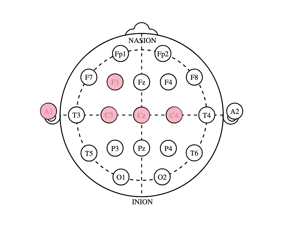
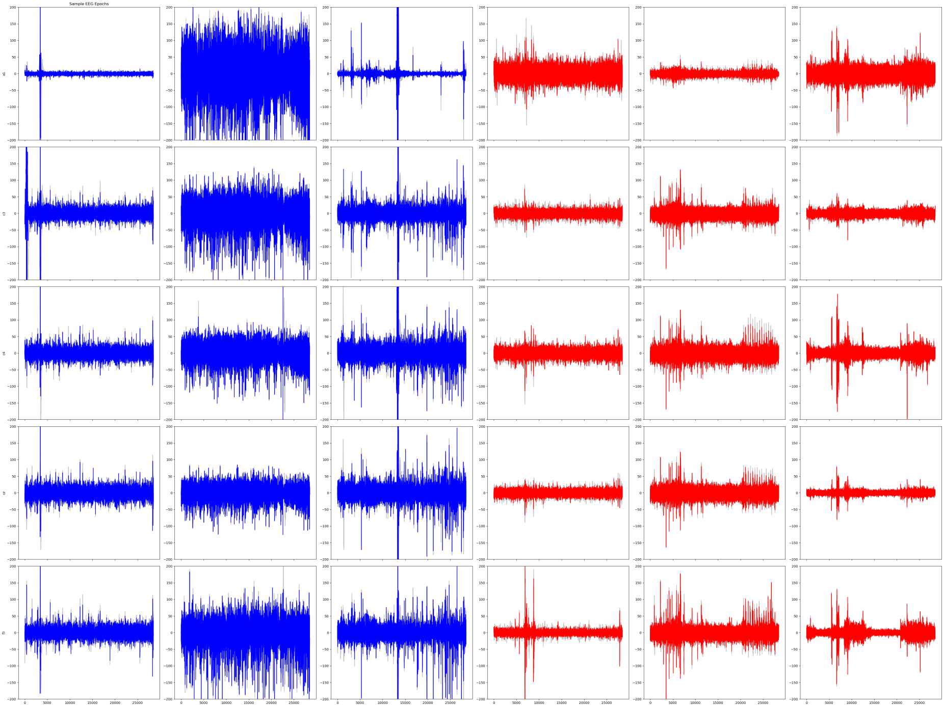
The data contains 411 recordings of people (epochs) per channel over 25 minutes at a sampling frequency of 200 Hz. Labels of healthy (visualized in blue) and epileptic (visualized in red) were given.
Methodology #
Data Cleaning #
We applied a bandpass filter to filter out unwanted noise, such as background electrical activity. We kept the frequencies 0.5 Hz to 10 Hz, which corresponds to the frequencies we are able to capture. See our code here.

A visualization of sample EEG waves across channels found that for the same epoch, wave patterns remained consistent across channels.
Feature Extraction #
Even with filtered data, the number of timepoints (28,500) is too many to fit into a model. Thus, we extracted statistical measurements (features) from the data, reducing computional costs of our models. The following features were extracted:
Basic statistical features like mean, median, range, quartiles, variance, standard deviation, skew, and kurtosis (measures the relative number of outliers).
Wave features like signal intensity, signal trend, zero crossing rate (number of times the signal changes signs), and number of peaks.
Spectral features (frequency domain features) like spectral centroid (frequency-weighted average), spectral bandwidth, spectral rolloff (85% cutoff rate), and peak frequency.
We also separated each EEG wave into its composite brain waves. Because our data was downsampled to 20 Hz, as per the Nyquist-Shannon Sampling Theorem, we are only able to accurately capture frequencies from 0-10 Hz. This allows us to evaluate delta (0.5-4 Hz), theta (4-7 Hz), and parts of alpha (8-12 Hz) waves. We did not have the data to evaluate beta (12-30 Hz) and gamma (30-100 Hz) waves. The low-frequency brain waves we did evaluate are associated with subconscious or relaxed brains states. We extracted basic statistical features regarding the composite delta, theta, and low alpha waves.
All together, we preliminarily extracted 41 features per electrode channel, 205 features in total.
Check out our code here.
EDA #
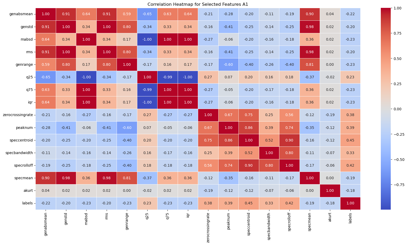
A correlation heatmap of all of the features we extracted for the electrode channel A1 reveals two main useful insights.
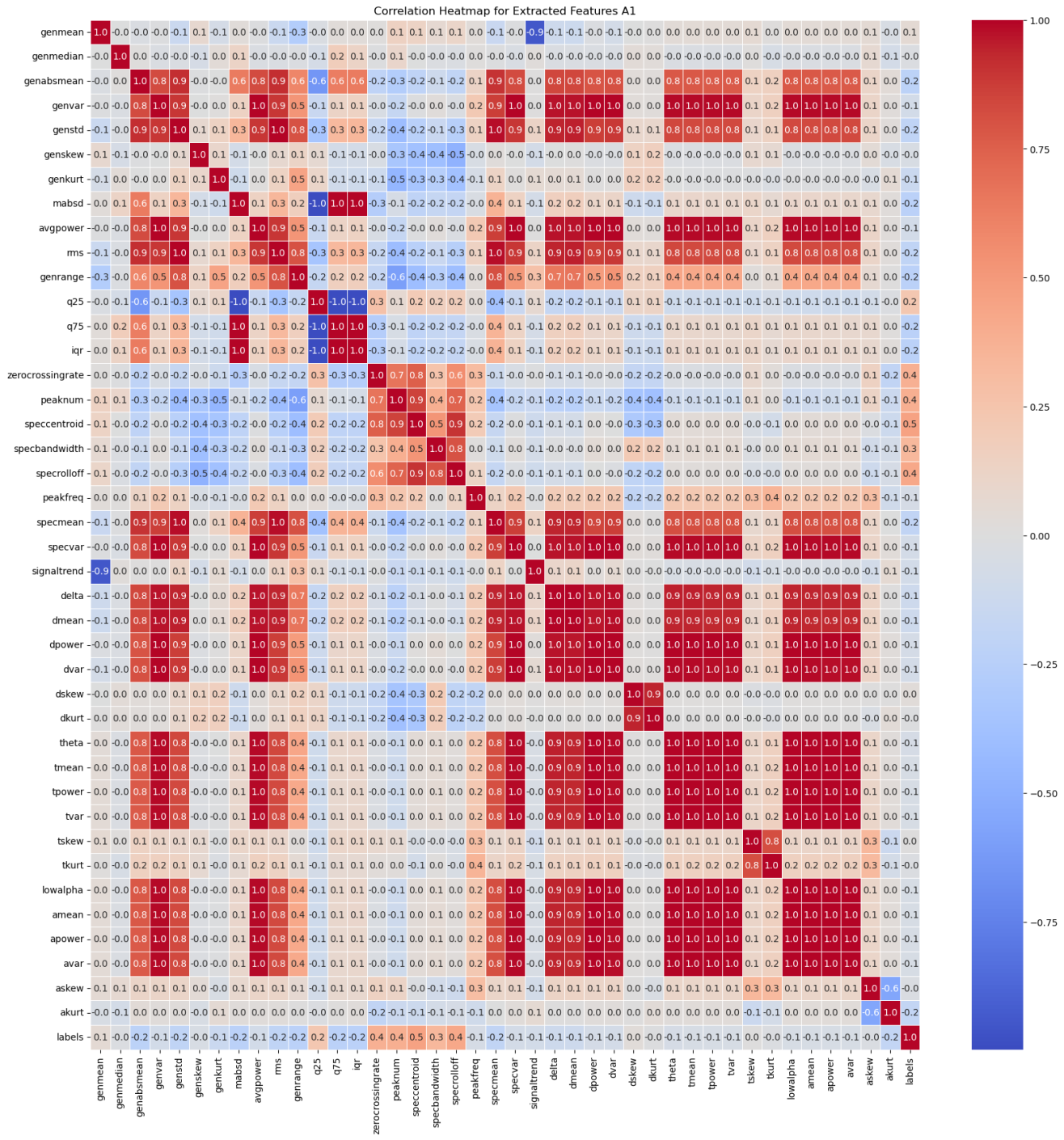
- The heatmap shows some features that might be more important to the final model. In particular, the zero crossing rate, number of peaks, spectral centroid, spectral bandwidth, and spectral rolloff have stronger correlations with the label (healthy or epileptic) compared to other features.
- Many features have a perfect linear correlation, or very weak correlation. As such, we can save computing power by selecting only the most important features to feed into our models.
Feature Selection #
We selected the top 15 features from each electrode channel using the F-Test, leaving us with a much more managable 75 features in total. The F-Test is a statistical test used to measure the significance of a feature compared to the label (healthy or epileptic).
Explore our code here.
A correlation heatmap of these selected features show that most variables with 0 linear correlation to the labels have been removed. As expected, the zero crossing rate, number of peaks, spectral centroid, spectral bandwidth, and spectral rolloff are all kept.
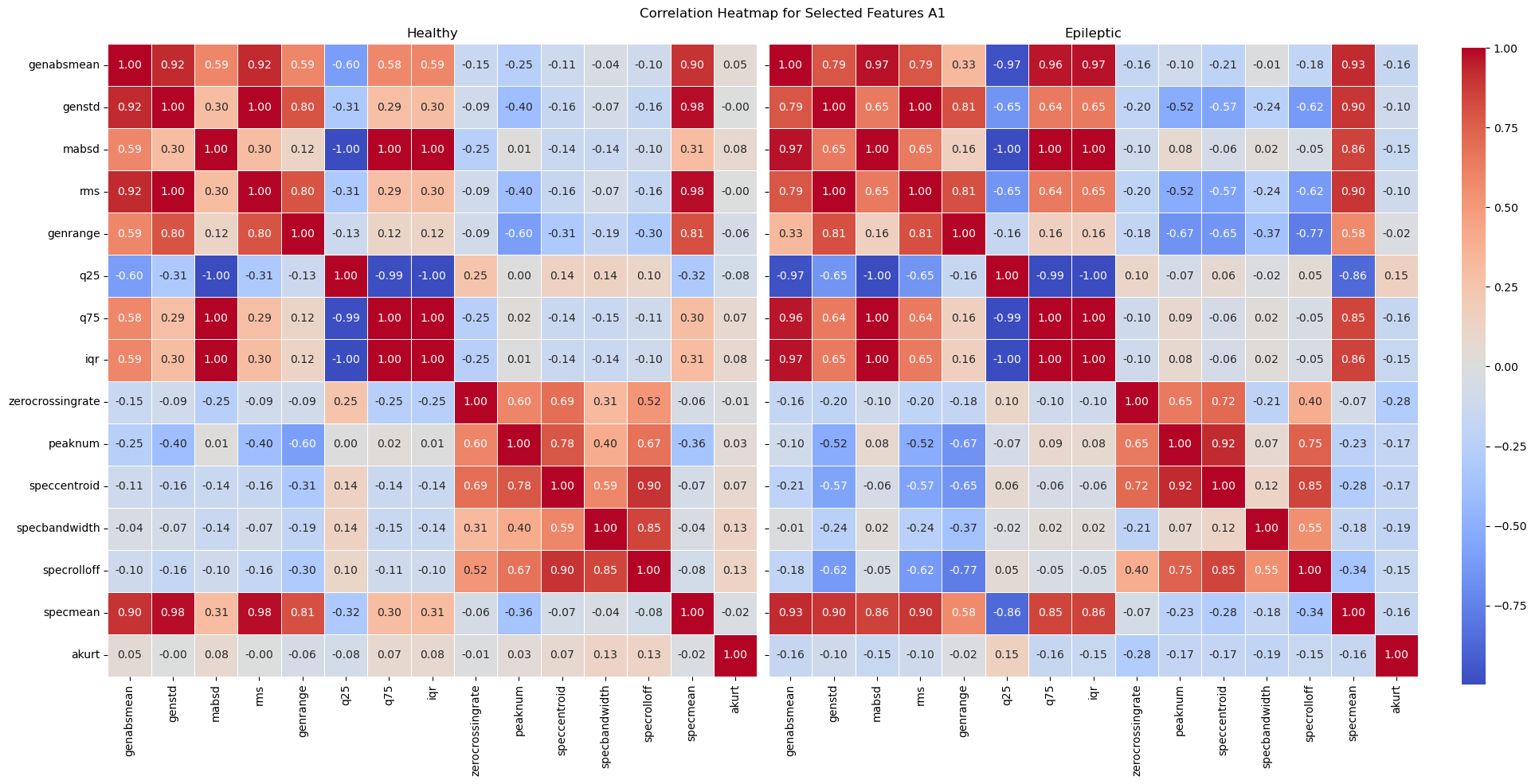
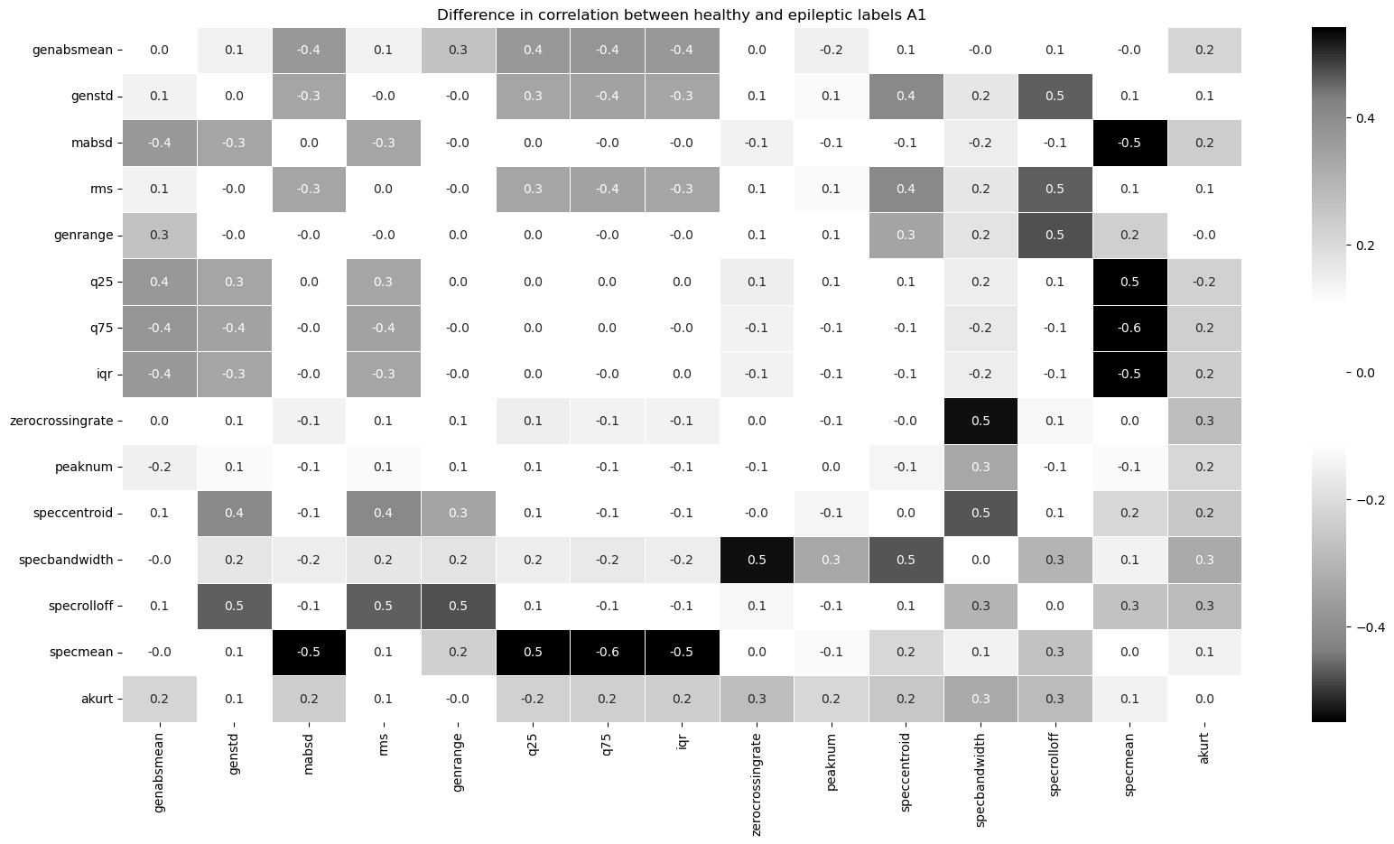
Some correlations between the spectral mean and basic statistical features are significantly larger for epileptic eeg samples compared to healthy samples. These correlations can be used to classify eeg signals in our models.
Modeling #
We compared multiple classes of models to see which would be the most effective. We tried 6 different models:
Logistic Regression: A parametric model that fits a “best-fit” line, then uses that line to calculate the probability of categorical outcomes (in this case healthy or epileptic). View our code here.
K-Nearest Neighbors (K-NN): A non-parametric model that classifies points based on the majority classification of their “k” nearest neighbors. In our model, “k” was optimized to 8. See our code here.
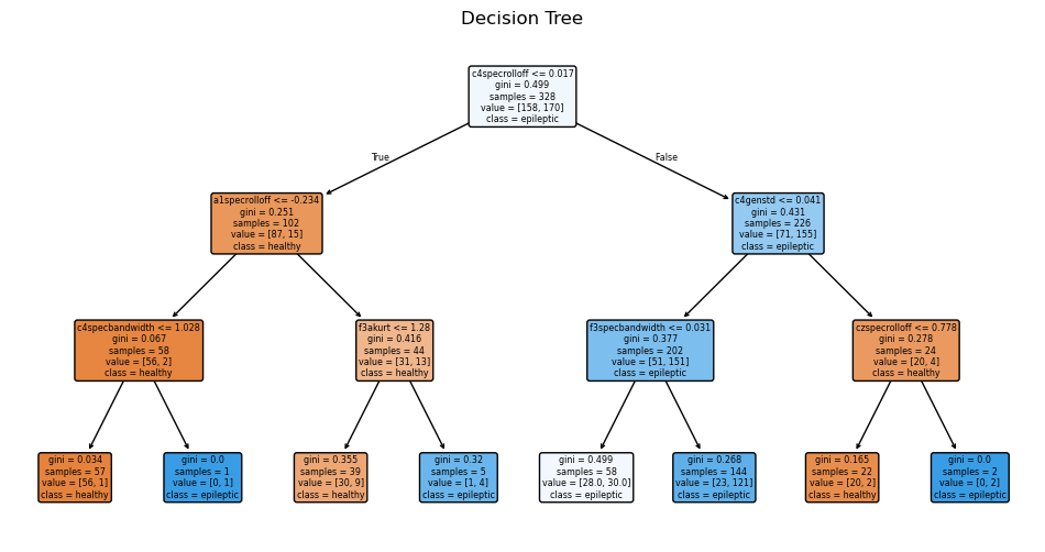
Decision Tree: A non-parametric model that makes a tree-like series of decisions conditionally classifying each instance. In our model, the depth of the tree was optimized to 3. Check out our code here.
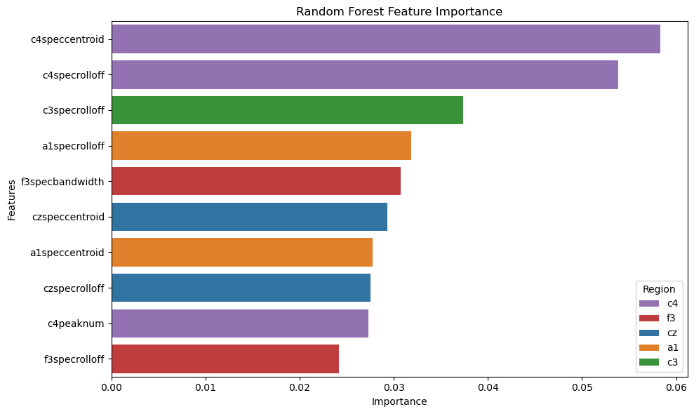
Random Forest: A non-parametric model that takes the average of many decision trees, each trained in parallel on a random subset of data, reducing overfitting. In our model, the maximum depth of each tree is optimized to 6 and the number of decision trees is optimized to 200. View our code here.
Gradient Boosted Classification Tree: A non-parametric model like random forest, but each tree is trained sequentially off of the errors of the last tree. In our model, the maximum depth of each tree is optimized to 3, the number of decision trees is optimized to 300, and the learning rate of each tree is optimized to 0.5. See our code here.
Support Vector Machine (SVM): A non-parametric model that finds the optimal hyperplane to separate data into classes. Our model uses a radial basis kernel to transform our data into a linearly separable form. Check out our code here.
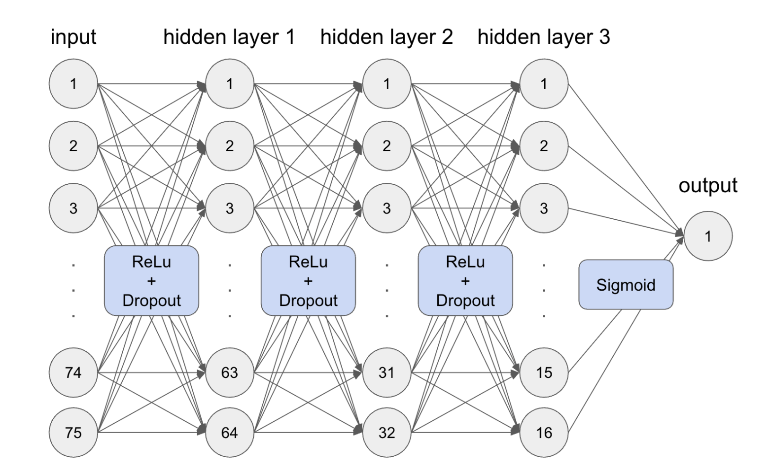
Multilayer Perceptron (MLP): A machine learning model and type of neural network. Our model consists of three hidden layers, bringing the feature dimensions from 75 to 64 to 32 to 16 to finally 1. Each hidden layer uses the ReLu activation function, and the output passes through a Sigmoid function to format it for binary classification. In our model, the dropout rate is optimized to 0.3, and the number of training epochs is optimized to 51. See our code here.
Results #
We used a few different metrics to compare how well our models perform:
Accuracy: A measure of how often the model predicts the label correctly (correct predictions/total number of predictions).
Precision: A measure of the accuracy of positive predictions made by the model (correct positive predictions/all positive predictions). In our case, precision measures the chance that someone actually has epilepsy if our model tells them they have epilepsy.
Recall: A measure of how well a model is of finding all positive (epileptic) cases (correct positive predictions/all positive cases). In our case, recall measures how many actually epileptic cases the model can diagnose as epileptic.
To us, recall is the most important metric, since undiagnosed and therefore untreated epilepsy can be very dangerous, sometimes even leading to death.
| Model | Logistic Regression | K-NN | Decision Tree | Random Forest | Gradient Boosted Regression Tree | SVM | MLP |
|---|---|---|---|---|---|---|---|
| Accuracy | 0.82 | 0.83 | 0.75 | 0.86 | 0.87 | 0.84 | 0.88 |
| Precision | 0.87 | 0.81 | 0.70 | 0.86 | 0.86 | 0.84 | 0.88 |
| Recall | 0.77 | 0.88 | 0.88 | 0.86 | 0.88 | 0.86 | 0.88 |
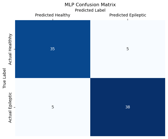
Across all metrics, the Multilayer Perceptron performed the best, identifying cases correctly 88% of the time, ensuring that the people it diagnoses as epileptic are actually epileptic 88% of the time, and catching 88% of actual epilepsy cases.
Discussion #
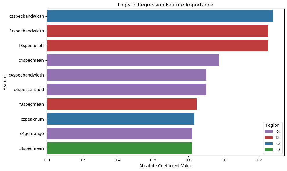
Although the Multilayer Perceptrons was most performant on this dataset, the decipherability of the model is one major drawback. The neural network acts as a “black box,” giving results that, although correct, are very uninterpretable. Looking into the other models, we find that their accuracy, precision, and recall are very comparable to that of the neural network, showing that the features we extracted from the data plays a much larger role than the archtecture of our models. Two models, Logistic Regression (82% accuracy) and Random Forest Classification (87% accuracy), provide easier ways to visualize which features are most important in classification.
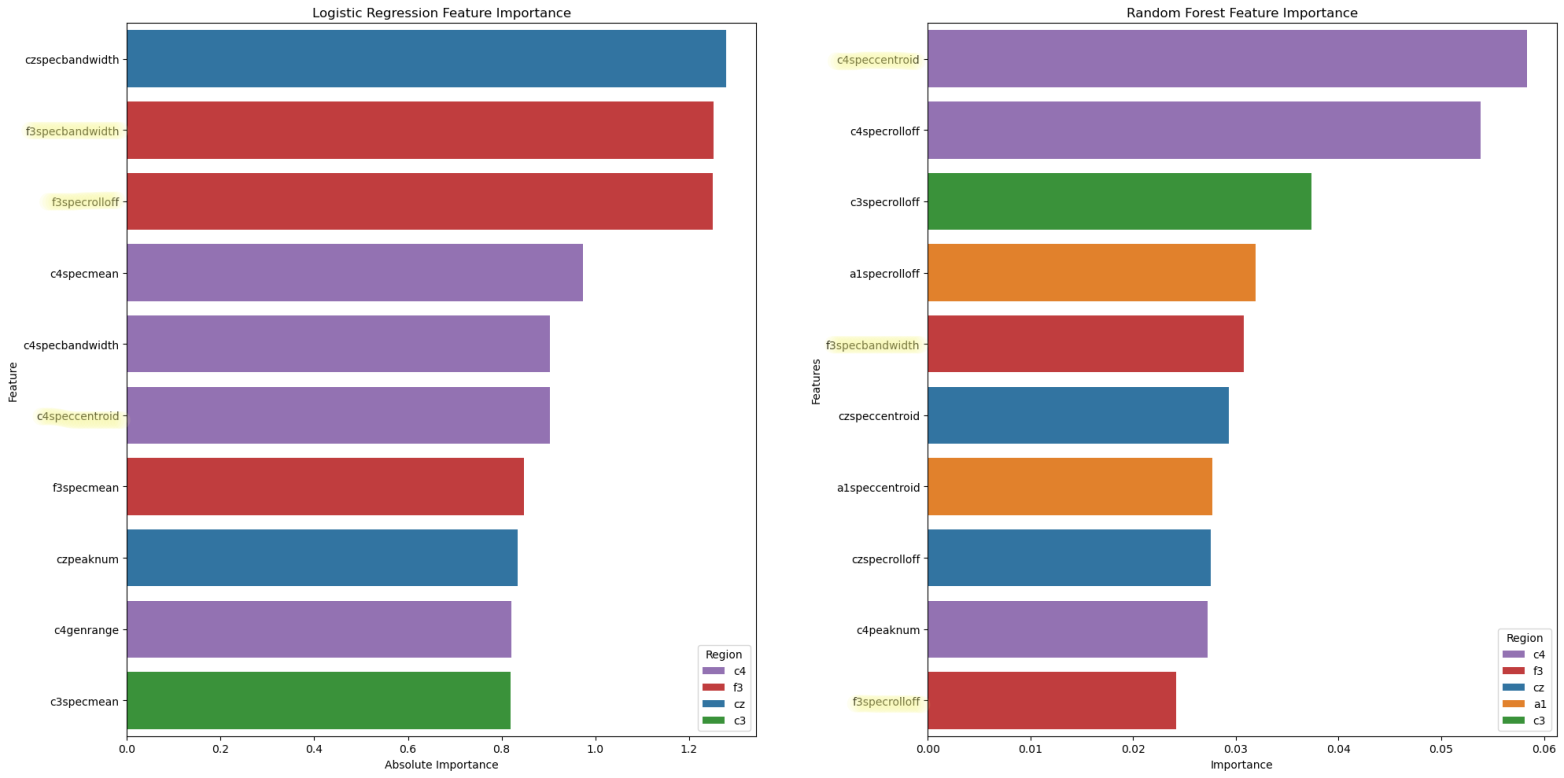
Spectral (frequency) features are the most considered across both models. C4 is the most important electrode channel, perhaps because it is the only electrode channel in our data that is placed on the right side of the brain.
In this project, we explored how to build an effective model with very limited (downsampled) data, which could have practical implications in areas that do not have the technical capibilities to collect the full range of EEG data. In the future, we hope to future explore data from other electrode channels as well as higher frequencies to create more accurate predictions that properly mirror how EEG data will be found in the real world.
See our entire workflow here.